It seems like almost every day I see a post on X, LinkedIn, or a blog about people canceling their OpenAI or Anthropic subscriptions because they can replace them with local LLMs. Here are two examples: a first day away from Claude Code (August 21) and a claimed $1,200/year coding-subscription replacement (September 1). I definitely think that open source models have come a long way since the days of Llama, so I wanted to try it myself. I already had the hardware and hoped I’d learn something new.
How to get started?
One of my favorite electronics retailers turned out to be the perfect place to start: Micro Center’s local LLM guide. In their guide, they have a simple table that assumes your local LLM will run at 4-bit quantization and a fixed 32k context window. Based on those assumptions, they show you a few options for the amount of GPU memory you will need to run an LLM of a particular size.
I kind of trust quantization in 2026, but 32k context? It seemed like an awfully small number compared to the 1 million tokens Opus shows me each time I use Claude Code. It’s obviously significantly smaller, but is it so small that it’s unusable? The system prompt, tool definitions, files, command output and conversation history all have to fit somewhere, but all these posts make it seem like it’s not an issue whatsoever.
This left me with a few questions. How practical is a 32k context window? Am I really limited to such a small context window, or can I scale it up to fit on my hardware without my generation speed slowing to a crawl? Finally, can I run several agents with the full context window configured and use OMAR (Open Multi Agent Runtime) to manage multiple agents, as that’s how I use Claude Code and Codex these days?
Spoiler: yes, I can do it all on hardware that costs under $3,500. On my AMD Ryzen AI Max+ 395, I got Qwen3.6-35B-A3B running with its full 262,144-token context window configured and available, eight times the 32k assumption from the guide. I use Pi as my coding harness, and I get one agent to generate about 57 tokens per second through llama.cpp, or 42 through vLLM. For these speed tests, I asked the agents to keep generating jokes. Finally, I pushed both backends to 32 concurrent agents to see where the experience stopped feeling useful because it was too slow.
In this blog post, I’ll explain how context consumes memory, why bandwidth and MoE vs dense models change token generation speed, and what happened when I started scaling to multiple coding agents through OMAR. While I will not cancel any of my subscriptions at this time, I hope that my experience can help shed some light on an area that, at least to me, felt too good to be true.
How much coding work fits in 32k?
A token is a chunk of text the model processes, which can be a word, part of a word, punctuation or whitespace. The tokenizer determines how the text is split, so the same code can take up different numbers of tokens in different models. I’ll use 32,768 tokens for 32k in the calculations below.
Pi turns out to be a great choice for a coding agent harness because it’s tiny and open source, so it’s simple to understand. Plus, it saves you money on taxes haha. Pi sends the LLM instructions about its role (the system prompt), descriptions of the tools it can call, and the task. As the agent works, it adds file contents, command output and its own responses to that history. In the request I captured, the initial prompt and descriptions of Pi’s four default tools already occupied about 1,640 tokens.
A one-line fix can involve a lot of code
I started with the first task in the SWE-bench Verified dataset: astropy__astropy-12907. SWE-bench contains real repository issues paired with their fixes. This issue concerns incorrect separability results for nested CompoundModel objects. The reference fix changes one line in astropy/modeling/separable.py.
To get an exact token count, I used the tokenizer for Qwen3.6-35B-A3B. Here is what the issue and three relevant files take up, before chat formatting or tool-result wrappers:
| Material inspected | Tokens |
|---|---|
| Issue description | 341 |
separable.py, where the fix goes | 2,580 |
test_separable.py, the existing tests | 1,553 |
core.py, which defines CompoundModel | 38,952 |
| Issue and all three source files | 43,426 |
Reading the issue, implementation and tests gives 4,474 tokens. Inspecting the complete module that defines the compound models brings the source material to 43,426. Add my captured Pi request’s approximate 1,640-token footprint and the working context is already around 45,066 tokens, before the agent adds explanations, edit calls or test output.
In practice, an agent usually reads sections of a file through tool calls. Those chunks still accumulate in the conversation. When the history gets too large, Pi compacts it into a summary so the agent can continue.
The agent also needs room to answer. In Pi 0.85.1, the default response reserve is 16,384 tokens. Compaction starts when the history exceeds the window minus that reserve, according to the versioned compaction code. Of course, one can configure this, but I’m not sure everyone who’s running local LLMs with Pi is aware of this setting.
| Configured window | Response reserve | Context threshold for compaction |
|---|---|---|
| 32,768 tokens | 16,384 tokens, Pi’s default | 16,384 tokens |
| 262,144 tokens (Qwen’s full context window) | 16,384 tokens, Pi’s default | 245,760 tokens |
Loading all that source would take 45,066 tokens, exceeding both Pi’s default compaction threshold and the entire 32k window. Carrying those reads together would require summarizing or discarding earlier material. With the full window enabled (for this particular LLM), the same material occupies about 17% of the context capacity.
How much context did real coding agents use?
To see what agents actually read, I counted the histories in 500 public SWE-bench Verified runs using Claude Sonnet 4 and mini-SWE-agent. mini-SWE-agent is a coding harness that lets the model run shell commands to read files, edit code and test changes. I counted the recorded message text before each model call with Qwen’s tokenizer, including the command output that came back.
The median task took 33 model calls and reached a peak history of 15,140 tokens. The largest reached 92,323 tokens.
| Recorded history exceeded | Tasks |
|---|---|
| 16,384 tokens, Pi’s default compaction threshold at 32k | 213 / 500 (42.6%) |
| 32,768 tokens, the entire 32k window | 25 / 500 (5%) |
| 245,760 tokens, Pi’s default threshold at full context | 0 / 500 |
For example, this Django middleware task took 58 model calls and reached 29,735 tokens. It would fit inside the entire 32k window, but it crosses the threshold Pi uses with its default response reserve. The Astropy task from the file-count example above reached just 11,913 tokens in its recorded run. Selective reads used much less context than loading all three files.
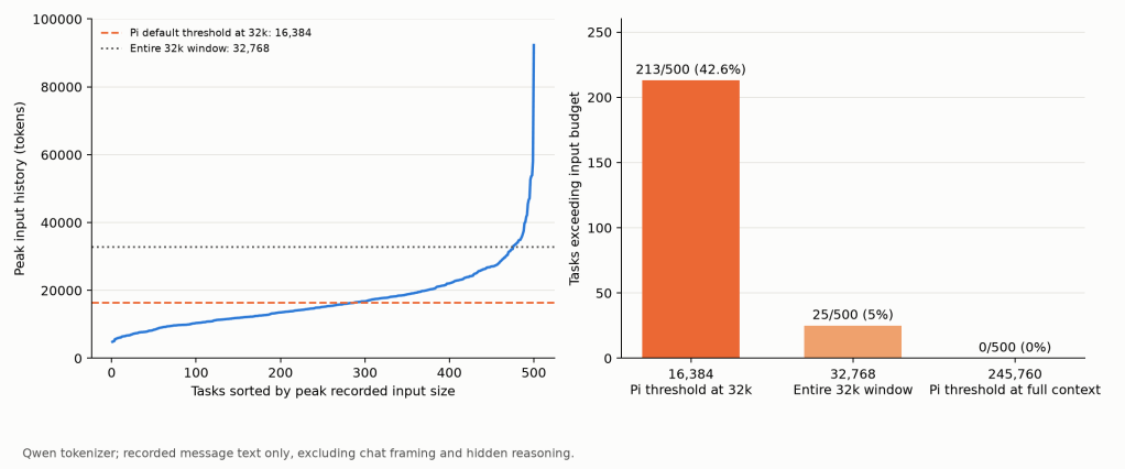
Those histories gave me a reason to want more context. First, I needed a model that ran at a speed I could use.
What I actually ran
My machine, the AMD Ryzen AI Max+ 395 (codename Strix Halo), can be found for just under $3,500. On my machine, I have 123 GiB of usable unified memory, physical RAM shared by the CPU and integrated GPU. The integrated GPU sees a 61.7 GiB shared-memory pool by default but that can be configured. I ran Ubuntu 24.04 with kernel 6.17.
Micro Center’s guide recommends 32GB or more for Qwen3.8 27B, with an 18.29GB footprint at 32k. The same guide gives 45.41GB at 256k. A 32GB RTX 5090 would fall short of that full-context footprint on its own. The cheapest listing I saw on NVIDIA’s marketplace was $5,049.99 for the graphics card alone. I’d still need a PC to put it in, adding to the total cost. A unified-memory system like mine or a MacBook Pro offers another way to get a larger memory pool.
The model fits. How fast does it run?
I used a 4-bit AWQ-quantized version of Qwen3.8-27B, following the guide’s 4-bit assumption. It is a dense model, meaning it uses nearly all its weights to generate each token. Quantization stores them at lower precision to reduce memory use. At exactly 4 bits per weight, 27 billion weights would take 13.5 GB, compared with 27 GB at 8 bits or 54 GB at 16 bits. Real checkpoints also include quantization scales and weights kept at higher precision, so their sizes differ from that simple calculation. Matt Bucci’s Qwen3.8-27B AWQ model page provides a downloadable 4-bit version and describes which components remain at 16 bits.
I used vLLM, the software that loads the model onto the GPU and serves generation requests. These tests use the vLLM performance settings described below. To match the guide, I configured a 32,768-token context limit and tested the server directly with one and ten concurrent requests. Each condition had three valid 45-second measurement windows using a short prompt. The dense model averaged 11.22 tok/s with one request and 26.71 tok/s in total with ten, or 2.67 per request. Per-request figures are the total divided by the request count.
Were these speeds acceptable? In this Reddit thread, some people are happy with 5 tok/s for chat, while others want at least 15–20. For coding, some put that number closer to 30–35 tok/s. Personally, I use 20 tok/s per agent as the lowest speed I find comfortable. Both results were below that. So what gives? I followed the guide and ended up with something too slow for how I use coding agents.
Memory bandwidth helped explain the single-request result. Most of the posts I’d seen focused on fitting the model into memory, without discussing how quickly the GPU could read it. During generation, the GPU uses the model’s weights to calculate the next token, then repeats the process for the token after that. A model this large cannot keep all its weights in the GPU’s small on-chip caches, so the GPU repeatedly fetches them from memory. Memory capacity, in GB or GiB, tells me how much fits. Memory bandwidth, in GB per second, tells us how quickly the GPU can fetch it. An agent working through OMAR wrote a small test that repeatedly reads GPU-accessible memory and measured about 240 GB/s.
That shared RAM is LPDDR5X system memory, while the 5090 uses dedicated GDDR7 graphics memory.
Why does the dense model read so much?
For my 4-bit Qwen3.8-27B checkpoint, counting the tensors used during text generation gave an estimate of 16.7 GB of weights per generated token. I summed the stored sizes of the checkpoint’s tensors, the arrays holding its model values. That includes the language layers’ packed 4-bit weights, their scales and the 16-bit output projection:
Weight bytes per token ≈ sum of stored tensor bytes used by the language layers + output projection ≈ 16.7 billion bytes = 16.7 GB.
The earlier 27B × 4 / 8 = 13.5 GB shortcut assumes every weight takes exactly four bits. Mixed precision and quantization data account for the larger estimate.
For one agent generating one token at a time, I can estimate the weight-read ceiling with:
Tokens per second ≈ memory bandwidth (GB/s) / weight bytes used per token (GB).
At 240 GB/s, reading 16.7 GB takes about 70 milliseconds, giving a weight-only ceiling of roughly 14 tok/s. Calculations, cache reads and GPU scheduling still take time. My measured 11.2 tokens per second was fairly close to that estimate. This explained why having enough RAM had not made generation fast: the GPU still had to read those weights for every token.
Could MoE speed this up?
A mixture-of-experts (MoE) model divides parts of its network into groups called experts. A small part of the network called a router selects which experts process each token. There are also shared parts of the model that every token uses. Qwen3.6-35B-A3B is an MoE model that has 256 experts per expert layer and selects eight for each token. It holds about 35 billion parameters in total, with roughly 3 billion active for a token (hence the name 35B and A3B). All the experts occupy memory, but generating one token reads the selected experts along with the shared weights. Several leading open-weight models use MoE too, including MiMo-V2.6-Pro, GLM-5.3 and Kimi K3.
The MoE’s tensor accounting gave approximately 2.3 GB of active weights per token with AWQ 4-bit quantization. At 240 GB/s, reading those weights takes about 9.6 milliseconds, giving a weight-only ceiling of roughly 104 tokens per second. I repeated the one- and ten-request tests with the same 32k limit, short prompt and three measurement windows per condition:
| 32k vLLM comparison | Dense Qwen3.8-27B | MoE Qwen3.6-35B-A3B |
|---|---|---|
| Estimated weight bytes read per token | 16.7 GB | 2.3 GB |
| Weight-only ceiling at 240 GB/s | About 14 tok/s | About 104 tok/s |
| Measured single-request generation speed | 11.22 tok/s | 42.34 tok/s |
| Measured total speed, ten requests | 26.71 tok/s | 126.41 tok/s |
| Average per request, ten requests | 2.67 tok/s | 12.64 tok/s |
The estimated weight bytes per token fell by about sevenfold, and measured generation was about 3.8 times faster. But why only 42.34 tok/s when weight reads alone suggest 104? The calculation leaves out compute, cache access and GPU scheduling. The dense model reached about 78% of its weight-only estimate, while the MoE reached about 41%. I used an earlier vLLM configuration to inspect the GPU work.
What would this look like on a MacBook?
As a quick comparison, an owner of a 128GB M5 Max reports about 25 tok/s with an 8-bit Qwen3.8-27B in this Reddit thread. That configuration has 614 GB/s of bandwidth (Apple’s specifications). Using the same bandwidth calculation with a nominal 27GB weight size gives 614 / 27 ≈ 22.7 tok/s, within about 9% of their report. That is only a rough comparison: their K_XL quantization mixes precisions, and I have not counted its weight reads per token. A base M5 MacBook Pro with 32GB of memory has 153 GB/s of bandwidth (Base M5 specifications). Using my 4-bit checkpoint’s 16.7GB weight estimate gives 153 / 16.7 ≈ 9.2 tok/s, before other costs.
If you want to see how tokens move through a language model, Jay Alammar’s Illustrated GPT-2 walks through it with diagrams. For more on the hardware side, the How to Think About GPUs chapter of How To Scale Your Model explains GPU compute, memory and bandwidth in more detail.
How I configured vLLM for these tests
The MoE reached about 41% of its weight-read estimate, compared with 78% for the dense model. Reducing weight reads leaves the other GPU work taking a larger share of the time.
AWQ stands for Activation-aware Weight Quantization; it uses sample inputs to guide how weights are reduced in precision. INT4 means four-bit integers. I used AWQ INT4 because vLLM has an optimized decoding path for it on this AMD GPU. This chip lacks native FP4 and FP8 matrix instructions; other weight formats can require emulation or fallback kernels.
The individual GPU programs that carry out model operations are called kernels. I used AMD’s rocprofv3 profiler to record GPU kernel launches while an earlier vLLM configuration generated 48 tokens. It recorded about 2,300 launches per token. Launching all those kernels takes work too. HIP graphs let the engine replay a prepared sequence of GPU operations, reducing the work needed to launch them. torch.compile turns model code into compiled operations, which can combine work into fewer kernels. Graphs alone gave no measurable single-agent gain in my probes, and compilation’s small gains at high concurrency could have been within run-to-run noise.
I also changed the settings for the kernel that combines MoE operations. This gave no useful improvement for one request, but helped with several requests at once, as the multi-agent results show.
vLLM also offers different implementations of attention, the operation that lets the model use earlier tokens when generating the next one. These implementations are called attention backends. I compared the default on this machine, ROCM_ATTN, with TRITON_ATTN. Switching to Triton made a large difference in the context-length test.
Can I run the full context window?
I also tried llama.cpp, another program for running local models, through Lemonade, which manages the model server. llama.cpp used Vulkan to access the GPU; vLLM used AMD’s ROCm 10.0.0 software stack, with PyTorch 2.12.0 and vLLM 0.27.1.dev5.
So far, I had kept the same 32k limit as the guide. Could I crank it up to the model’s full context window and still get usable speeds? I configured both engines for Qwen’s native 262,144-token limit, eight times the guide’s 32k. How much extra memory would that need?
Where does the context go?
Increasing the context window leaves the model’s weights the same size, but requires room to remember more tokens. Each full-attention layer calculates keys and values, numerical representations it uses to look back at earlier tokens. The engine saves these in a KV cache so it can reuse them during generation. Twice as many tokens means twice as much of that cache.
I used eight-bit cache formats: q8_0 in llama.cpp and fp8 (floating point) in vLLM. llama.cpp also used flash attention, which reduces memory traffic during attention.
The weights are learned numbers loaded from the checkpoint; the keys and values are intermediate results calculated from the current history. The engine unpacks the weights for computation and stores those results separately, so their storage formats do not have to match. Lower cache precision saves memory but introduces its own rounding error. Both llama.cpp and vLLM let me choose it separately from the weight format.
Only 10 of this model’s 40 layers use full attention. The others use Gated DeltaNet, which carries a running state updated with each token instead of keeping an attention-cache entry for every token. That hybrid architecture makes a large context window much cheaper to hold.
The cache is split into groups called KV heads, each holding a fixed number of values per token. The KV-cache calculation for one history is:
Cache bytes = tokens × full-attention layers × KV heads per layer × values per head × 2 (key and value) × bytes per value.
Qwen3.6-35B-A3B’s model configuration gives 10 full-attention layers, two KV heads and 256 values per head. With fp8’s one byte per value, that is 10 × 2 × 256 × 2 × 1 = 10,240 bytes per token, or 10 KiB.
| Tokens in one history | 16-bit KV cache | fp8 KV cache |
|---|---|---|
| 32,768 | 0.625 GiB | 0.3125 GiB |
| 262,144 | 5 GiB | 2.5 GiB |
So going from 32k to the full window needs eight times the attention-cache capacity. These figures cover the stored keys and values; q8_0 also stores quantization scales, so it takes slightly more space than fp8. The engine still needs memory for weights, working buffers and the other layers’ state.
How does this compare with what I measured? llama.cpp used about 24.0 GiB of GPU-visible memory with the full context configured. Its weight file was 20.2 GiB, and an eight-bit attention cache for the full window takes roughly 2.5 GiB, plus quantization scales for q8_0. Together, those account for most of the measured allocation, with additional space needed for the other layers’ state and working buffers. This is a rough memory budget; I measured the whole engine, not the cache in isolation.
vLLM reserved 52.5 GiB, controlled by its memory-utilization setting. That is a pool for weights, cache and working memory, rather than the memory cost of one full-length history. Both engines fit within the GPU’s 61.7 GiB pool.
llama.cpp calls its concurrent-request positions slots. I configured 32 so it could serve up to 32 agents at once. Each agent has its own token history.
llama.cpp’s unified KV cache shares the allocation across slots; adding 32 slots does not reserve 32 copies of the full context window. Separate histories still consume cache space as they grow. vLLM reserves its memory pool ahead of time, so increasing the context limit or filling more of the cache need not increase the memory shown by a system monitor. It uses more of the existing pool.
Settings for the full window
GGUF is the file format llama.cpp uses for the model weights; MXFP4_MOE names the quantization variant I chose. This file mixes formats: some expert weights use MXFP4, others use Q5_K or Q6_K, and the attention and shared weights use Q8_0. The engines used different quantized weights and cache formats, so these results compare the complete setups.
| Setup | llama.cpp through Lemonade | vLLM |
|---|---|---|
| Backend | Vulkan | ROCm with TRITON_ATTN |
| Weights | MXFP4_MOE GGUF, 21.7 GB | AWQ INT4, 20.3 GB |
| Model’s native context limit | 262,144 tokens | 262,144 tokens |
| Configured context limit | 262,144 tokens | 262,144 tokens |
| KV cache format | q8_0 | fp8 |
| Concurrent requests | Up to 32 slots | Up to 32 requests in the sweep |
| Execution settings | Flash attention, unified KV cache | torch.compile, HIP graphs, tuned MoE configuration |
These are the vLLM launch options for the context limit, cache format, memory pool and attention backend:
--max-model-len 262144 \--kv-cache-dtype fp8 \--gpu-memory-utilization 0.85 \--attention-backend TRITON_ATTN
Would a longer context slow generation to a crawl?
The window fit in memory, but generating against a longer history means more attention work. Switching attention backends had taken a single Pi agent from about 19 to 41.7 tok/s, a 2.2× improvement. I compared both backends and llama.cpp with progressively longer prompts.
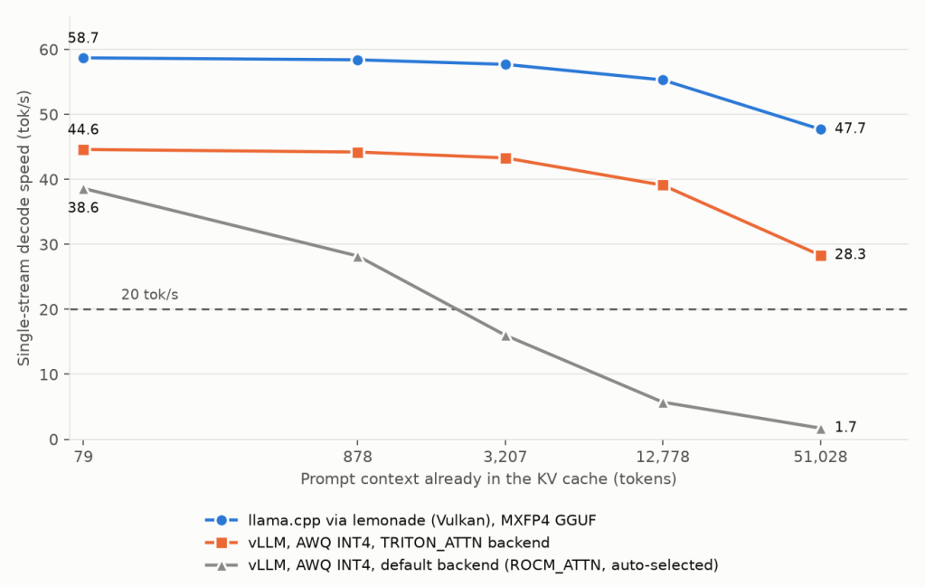
| Prompt tokens already in context | llama.cpp | vLLM with TRITON_ATTN | vLLM with default ROCM_ATTN |
|---|---|---|---|
| 79 | 58.7 | 44.6 | 38.6 |
| 878 | 58.4 | 44.2 | 28.2 |
| 3,207 | 57.7 | 43.3 | 16.0 |
| 12,778 | 55.3 | 39.1 | 5.7 |
| 51,028 | 47.7 | 28.3 | 1.7 |
I measured generation speed in tokens per second for one request using greedy decoding, which chooses the most likely next token at each step. These speeds exclude the time spent processing the initial prompt, called prefill. The vLLM context sweep used torch.compile and the default MoE configuration, rather than the tuned configuration used in the final agent sweep.
At that point, the default vLLM backend was producing 1.7 tokens per second. The alternative attention backend produced 28.3, and llama.cpp produced 47.7. A short-prompt demonstration would have hidden most of this difference.
Looking at the source gave me a possible explanation. With this model’s attention settings and fp8 cache, the default backend could not use ROCm’s specialized attention kernel. Its fallback scanned the cache with little work split across the GPU for each request. TRITON_ATTN split that scan into more segments. I did not isolate how much of the measured improvement came from that mechanism, but the change in the context curve was clear.
How many agents could I actually use?
In the 32k baseline, ten simultaneous requests reduced the average speed available to each one. I tested both engines with up to 32 Pi agents through OMAR, now with the full context configured.
Using the same 20 tok/s comfort threshold from the initial speed comparison, the average per-agent speed stayed above it through six agents with llama.cpp and four with vLLM.
I used Pi 0.85.1 with its four default tools. OMAR spawned and monitored separate Pi sessions under an Executive Assistant, the coordinator managing the agents, and the local server supplied the model. Each agent made one long streaming request asking for jokes, keeping them generating simultaneously without pauses for file reads, commands or new prompts.
I measured 45-second windows with the intended number of requests generating and no new prompts being processed. Every llama.cpp slot advanced; vLLM’s global counter could not establish individual stream speeds.
I tested 11 agent counts on each engine. One vLLM window at 12 agents stalled and was retried.
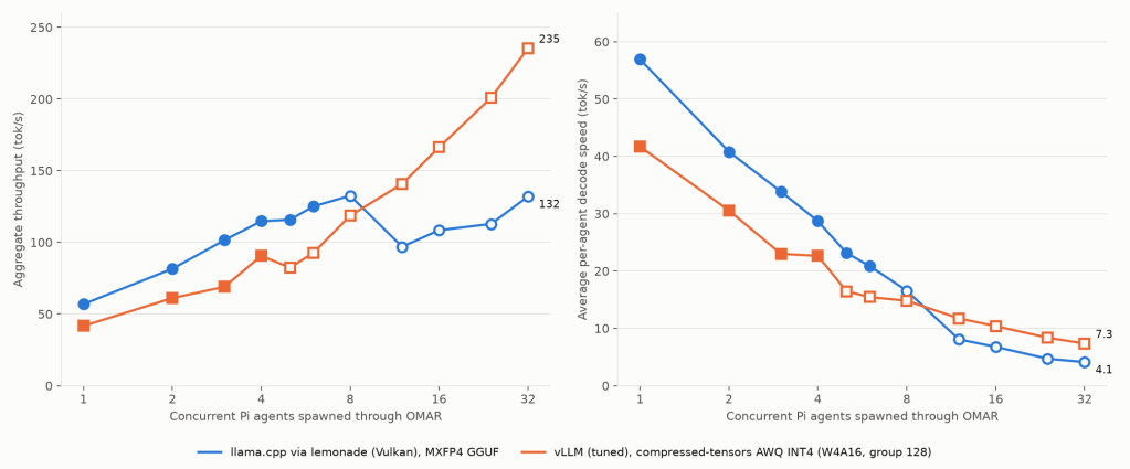
| Concurrent agents | llama.cpp total tok/s | llama.cpp tok/s per agent | vLLM total tok/s | vLLM tok/s per agent |
|---|---|---|---|---|
| 1 | 56.9 | 56.9 | 41.7 | 41.7 |
| 2 | 81.6 | 40.8 | 61.1 | 30.6 |
| 4 | 114.8 | 28.7 | 90.6 | 22.6 |
| 6 | 125.0 | 20.8 | 92.6 | 15.4 |
| 8 | 132.5 | 16.6 | 118.6 | 14.8 |
| 16 | 108.5 | 6.8 | 166.3 | 10.4 |
| 32 | 132.0 | 4.1 | 235.4 | 7.3 |
I then compared how compilation, tuning the GPU kernel that runs the experts, and changing the attention backend affected performance as I added agents.
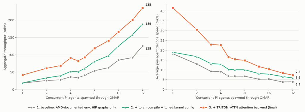
A separate four-agent comparison with TRITON_ATTN measured 95.7 versus 55.3 aggregate tok/s with the custom versus default MoE settings.
At 32 agents, vLLM’s 235.4 tok/s total came to 7.3 tok/s per agent on average; llama.cpp averaged 4.1. Both were below my 20 tok/s threshold.
Why did adding the ninth agent make it slower?
The main scaling chart had another surprise: speed did not change smoothly as I added agents. llama.cpp’s total dropped as I went past eight agents. A finer sweep measured 136.5 tokens per second at eight and 85.7 at nine.
I repeated the test by sending requests directly to the model server over HTTP, removing Pi and OMAR from the path. The drop remained: 147.2 at eight requests, then 93.6 at nine.
The server processes active requests together in a batch, generating one token per request in each decode step. In the installed llama.cpp build (b10723), the Vulkan backend switched kernel paths above eight tokens per step. A ninth active agent crossed that threshold. A per-operation profile on a Q8_0 version of the same model showed MoE matrix operations growing from about 24 to 35 milliseconds per step, and dense matrix operations from 18 to 32. Together they accounted for about 85% of the added step time.
vLLM had a smaller dip when moving from four to five agents. The HIP graphs described earlier were prepared for particular batch sizes, including four and eight. Five requests were padded to use the graph prepared for eight, paying much of that larger step’s cost while producing only five tokens. That fits the observed staircase, although I did not test it directly by capturing every batch size.
What did 32 agents look like in practice?
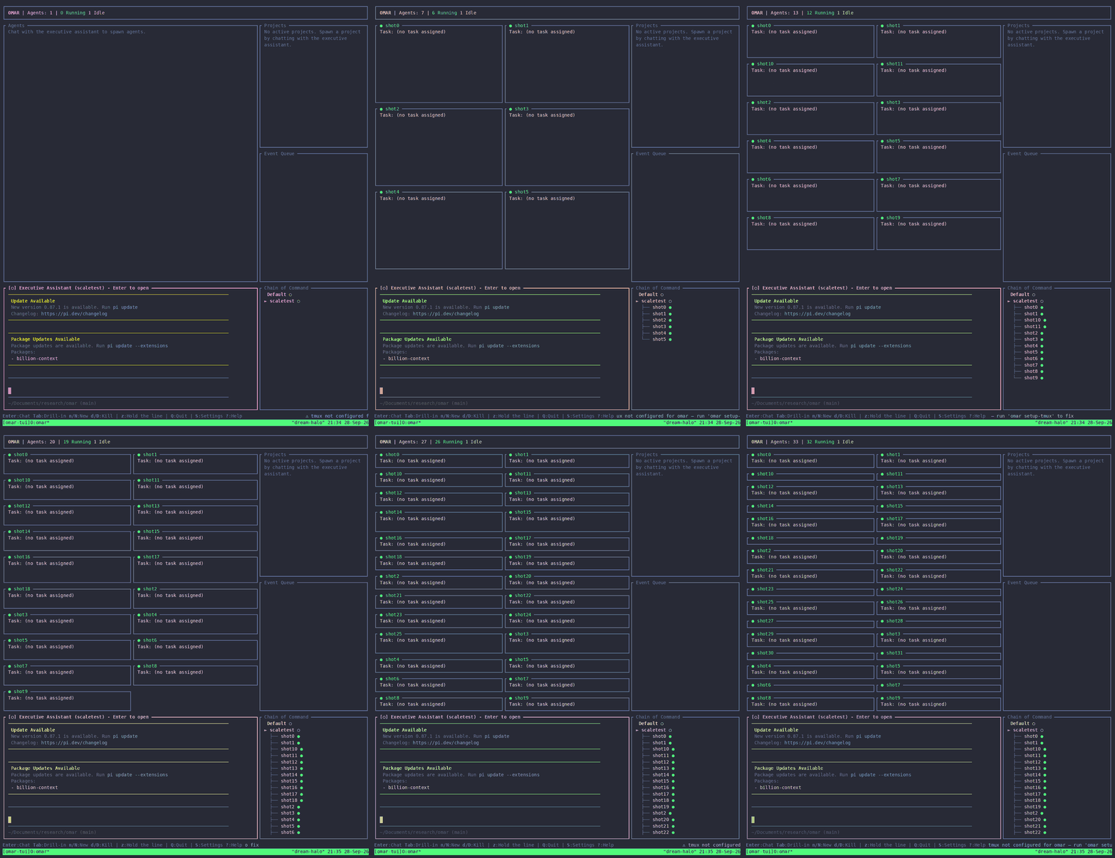
All agents shared one model server. GPU-visible memory stayed flat as I added them:
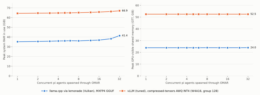
The sweep with the full context configured used one valid 45-second window for most agent counts. Repeating the 12-agent llama.cpp level gave 103.3 rather than 97.0 tok/s, so I would not choose an engine on a difference of a few percent.
Which engine would I use?
| Workload | Choice supported by these measurements |
|---|---|
| One interactive agent | llama.cpp: 56.9 tok/s, versus 41.7 for vLLM with these settings |
| A few agents, aiming for at least 20 tok/s per agent on average | llama.cpp: six agents met my threshold; vLLM met it through four |
| A larger group where total output matters | vLLM with these settings: 235.4 aggregate tok/s at 32 agents, versus 132.0 for llama.cpp |
I’d get more use out of six llama.cpp agents averaging about 21 tok/s than 32 vLLM agents averaging about 7. But these tests kept the agents generating jokes. I still need to see whether this setup can handle my daily coding work, such as building new OMAR features.
Qwen3.6-35B-A3B scores 18 on the Artificial Analysis Intelligence Index with reasoning enabled, matching GPT-6 Luna without reasoning. GPT-6.1 Sol at xhigh scores 51, and Opus 5.5 at xhigh with default fallback scores 56. Those are broad benchmark scores, and I haven’t evaluated my quantized setup’s coding ability, but that is a substantial gap to investigate.
That brings me back to those posts about canceling subscriptions. What coding work did their local model actually finish, with how much context, and how much did they have to correct? I got a full context window and several agents running at speeds I can use. I have no intention of canceling my subscriptions, but hopefully this gives you a better idea of what it takes to make local LLMs useful. A handful of agents working together on my own hardware is still pretty cool.
If you found this post useful in your research or work, please cite it as:
@misc{elmaaroufi2026localllms, title = {My experience running local {LLMs}}, author = {Karim Elmaaroufi}, year = {2026}, url = {https://kael.tech.blog/?p=299}}


Leave a Reply