Earlier this year, I coauthored a paper with AMD introducing Robotics Harness Optimization (RHO). In RHO, we use evolutionary search to improve robot policies that are whole code repositories. We tested it on repositories that both excluded and included LLMs at inference. The former are static codebases and are akin to what robotics engineers ship to companies as integration solutions while the latter are what researchers have been exploring through Code-as-Policies (CaP).
A few weeks after we released RHO, a new approach came out: Graph-as-Policy (GaP). In GaP, humans write skills (nodes) and LLMs merely have to stitch them together (connect them with edges). So naturally I was asked: can RHO optimize a graph? 🤔
In the rest of this post, I’ll share what happened when I applied RHO for fifty generations over an example graph from the GaP codebase. TLDR:
Graph-as-Policy
Graph-as-Policy (Chen et al., arXiv:2607.05369) replaces end-to-end policies (think RL trained policy or a VLA) with a directed computation graph whose nodes are individually meaningful skills: observe, perceive, compute a grasp, move, release. Their project page puts it plainly: the graph is the policy.
These graphs, like CaP before them, exhibit some interesting properties. First, the policy is source code you can read and diff, so a change can be quoted in lines. Next, failures localise to a named stage instead of somewhere unknown in a neural network. Lastly, edits are cheap, local, and searchable. Our evolutionary search process can propose “add a node” and score it without needing to collect demonstrations.
The starting graph from the GaP repo has twenty nodes (eighteen inside three subgraphs, plus the done and abort terminals), wired by conditional edges that route on each subgraph’s exit value.
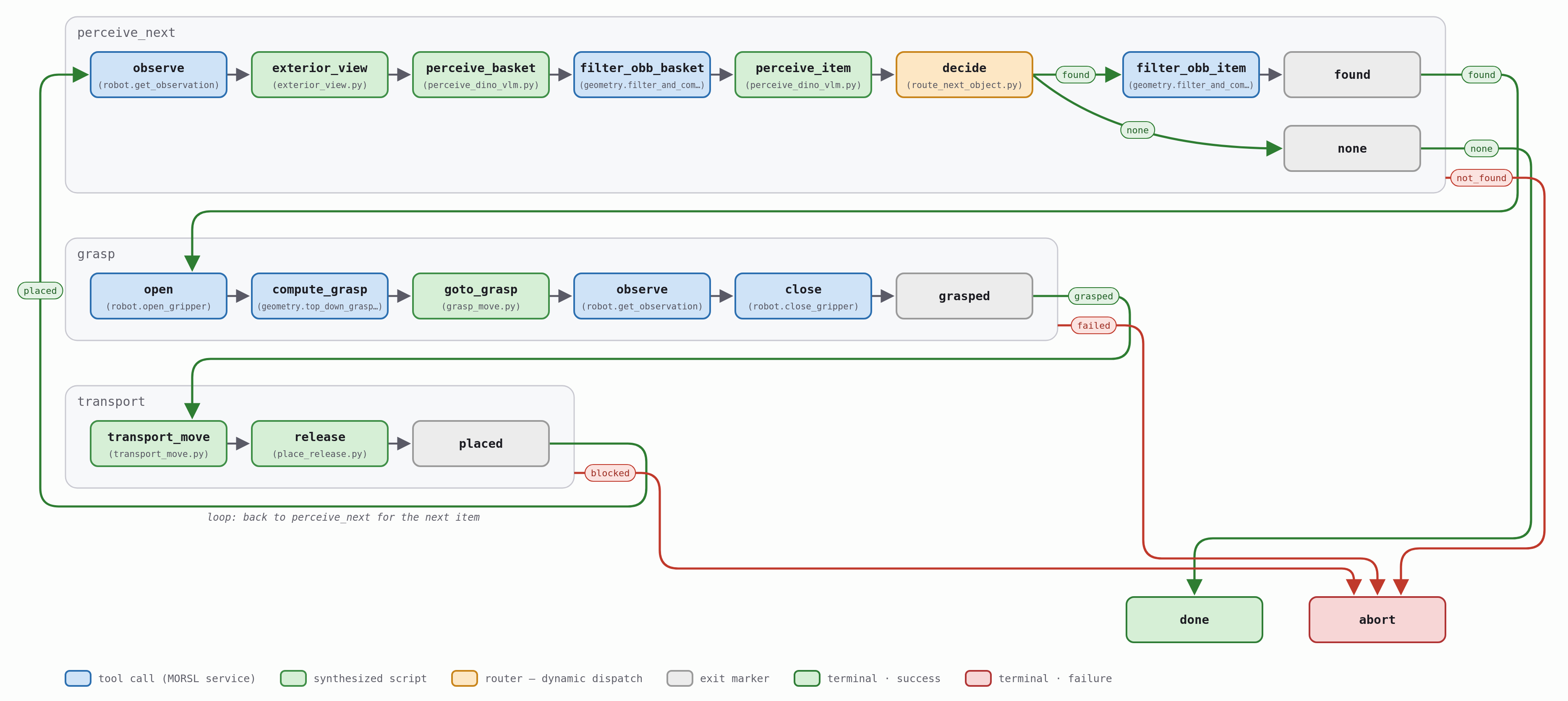
perceive_next and looks again. Only after perceiving again does decide ask whether it is finished, by polling the simulator’s sim.check_success. Blue nodes are tool calls into GaP’s services, green are LLM synthesized scripts, amber is a router that dispatches on an exit value.And here is the query it perceives with:
# seed/graphs/grocery_packing/workflow.json, perceive_item node inputs
"object_name":        "grocery item",
"object_description": "a packaged grocery product such as a can, box,
                       carton, jar, or bottle. Never the wicker basket
                       or storage container that the items are being
                       packed into."
The experiment
The example from the GaP is grocery packing with a simulated Franka Panda arm. It uses a LIBERO scene with a table of groceries, one wicker basket, and a sentence as the input task/prompt statement: “Pick the cream cheese and place it in the basket.” Sounds easy right? Well it’s 2026 and there’s a bunch of people focused on laundry folding humanoids so here we are. In this LIBERO setup, the hard part is object localization: the products are 20–40 pixels across in the camera image and several look alike. The robot has no privileged access to where anything is. It gets wrist and exterior color and depth cameras, and the sole prompt sentence.
Besides this introductory task, we look at the full benchmark which has eleven instructions. Ten of them name a single item: alphabet soup, cream cheese, salad dressing, BBQ sauce, ketchup, tomato sauce, butter, milk, chocolate pudding, and orange juice. The job is to put that one item in the basket. Nothing else. The eleventh says “Pick all the objects and place them in the basket,” and it’s played across ten different table layouts.
Here’s the interesting thing. The exemplar graph never actually reads the instruction. Its perception node is hardcoded to query for “a grocery item,” so it finds one (confidently, at a detection score of 0.95 to 0.98 whether it is right or wrong), carries it to the basket, fails the completion test, and loops around to try another. It’s basically playing process of elimination. On the ten single-item instructions it grasps an average of 4.17 objects to complete a task that needs exactly one.
To see what RHO would do with this, I ran two searches of fifty generations each over that same starting graph. I used codex with GPT-5.6 Terra on high reasoning with up to 200 turns as my mutator. In the first experiment, Compose-Only, I allow the agent to only add new nodes and rewire the graph, but has to use the human-written skills as given. This is in the original spirit of GaP. Compose-and-Edit can do all of that and also rewrite the skills themselves. So the question is: does an LLM that’s only allowed to stitch skills together lose anything compared to one that can open them up?
We implemented RHO on HELIX rather than another evolutionary optimizer because HELIX allows for mutating multi-file repositories with full agentic coding sessions rather than single-text artifacts with LLM API calls. The coding agents work in an isolated git worktree over many turns reading, grepping, running commands, interacting in the robot simulator. Each candidate is scored on held-out task instances (seeds or scene layouts) and the better ones are retained.
In HELIX, we can express the difference of the two experiments in three lines of configuration:
# Experiment 1 - Compose-Only: may rewire the graph, may not edit the shared skills
registries = ["…/open-robot-skills"]

# Experiment 2 - Compose-and-Edit: same freedoms, plus its own writable skill copy first
registries = [".", "…/open-robot-skills"]
As one might expect, more freedom to search and try things might result in a longer search and ultimately more tokens. Here’s what I spent and how long this took me on an NVIDIA DGX Spark:
| Experiment | Cost | Input | Output | Time | Admitted |
|---|---|---|---|---|---|
| Compose-Only | $14.39 | 42.7M | 197K | 34.1 h | 10 / 50 |
| Compose-and-Edit | $22.83 | 70.5M | 282K | 42.5 h | 9 / 50 |
Experiment 2 cost 65% more input tokens and 8.4 more hours for the same fifty generations.
Both searches figured out that the robot needed to read the instruction. Only one of them also learned to check whether the task was done right after placing the item, which turned out to matter a lot.
Results
Following the GaP paper, I report throughput: successes per hour, or success rate divided by cycle time.
| Policy | Success rate (95% CI) | Cycle time | Successes/hr (95% CI) | vs. baseline |
|---|---|---|---|---|
| Baseline | 67/100 · 0.57–0.75 | 144.9 ± 95.9 s | 16.6 [13.2–20.7] | 1.00× |
| Compose-and-Edit | 97/100 · 0.92–0.99 | 68.0 ± 15.1 s | 51.3 [48.2–54.0] | 3.08× |
| Compose-Only | 96/100 · 0.90–0.98 | 39.4 ± 19.9 s | 87.6 [76.9–97.8] | 5.27× |
The two RHO experiments are indistinguishable on accuracy; their success-rate intervals overlap almost completely. However, their throughputs tell a different story: the intervals do not overlap at all.
Here’s what each search built.
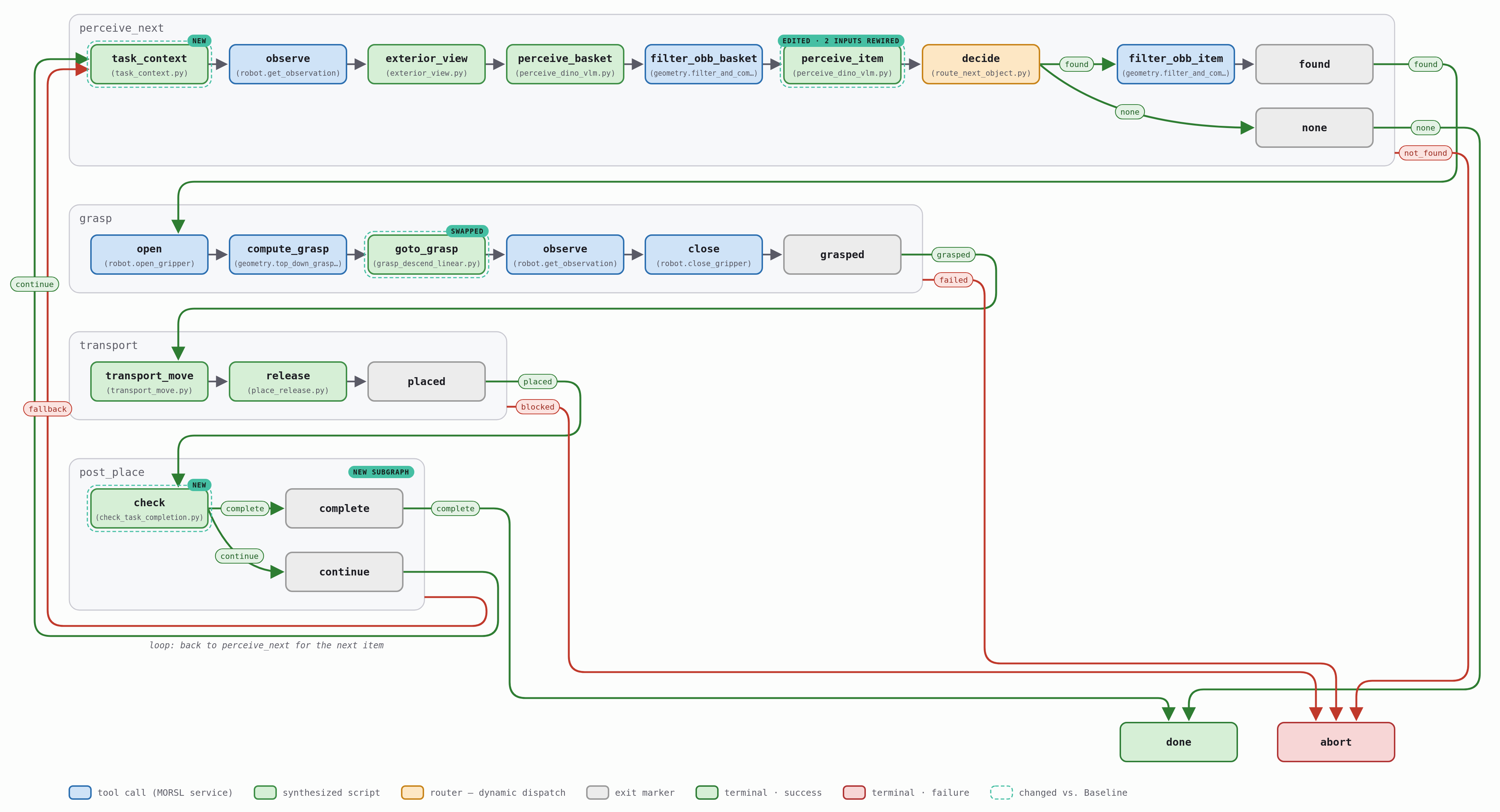
task_context runs before perception and resolves the target out of the instruction; check, in the new post_place subgraph, asks whether the task is done and exits instead of looping back for another perception pass. The grasp swap pulled an existing script in from the shared registry unmodified. This is exactly what Compose-Only is allowed to do.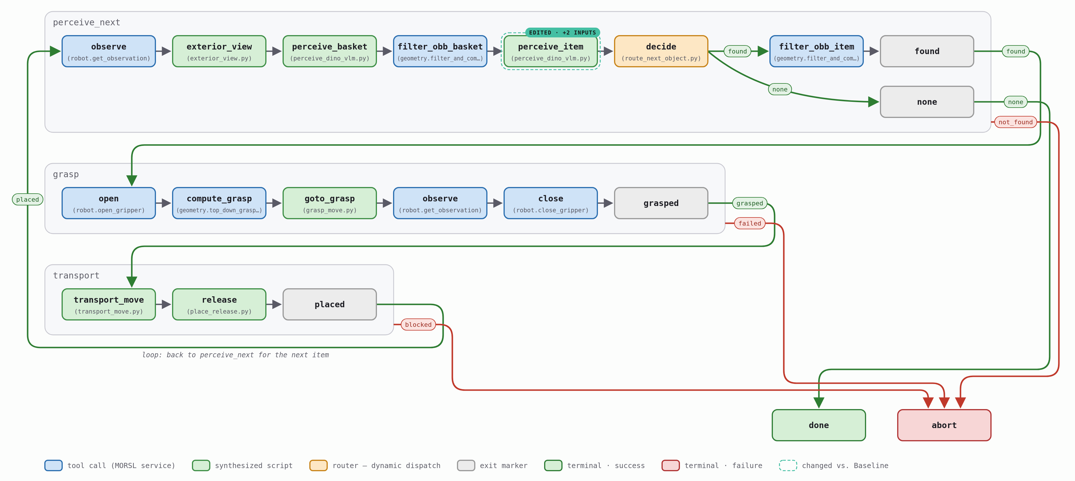
perceive_item, which switch on code the search added inside the perception script itself.Finally, let’s see the benchmark tasks and the results but with videos! All three GaPs side by side on the same starting task instance. All three receive the same 3x rendering speedup so anyone that finishes first, is actually that much faster than the others.
“Pick the alphabet soup and place it in the basket”
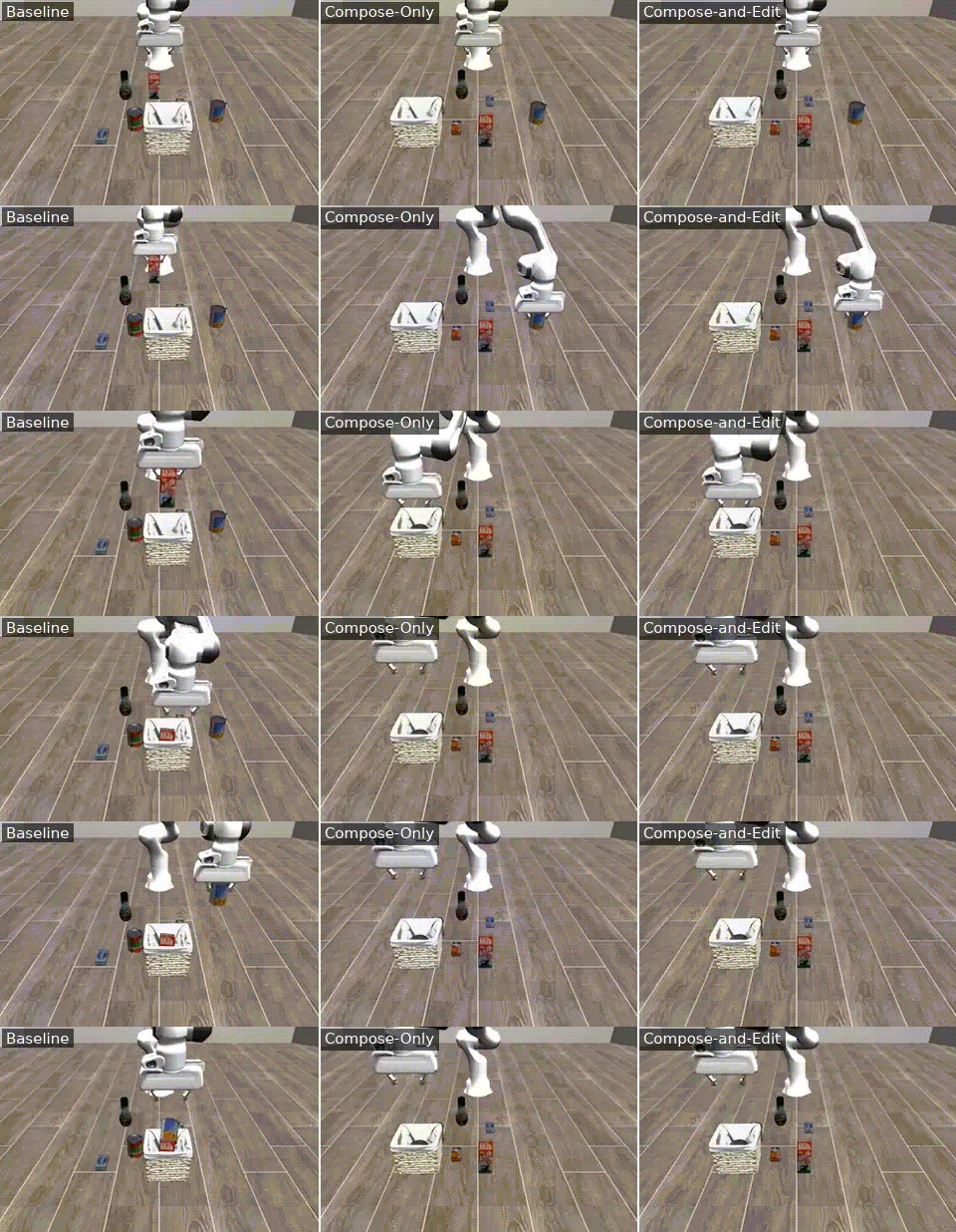
| Baseline10/10 · 118 s · 30.4/hr | Compose-Only9/10 · 44 s · 73.4/hr | Compose-and-Edit9/10 · 80 s · 40.3/hr |
“Pick the cream cheese and place it in the basket”
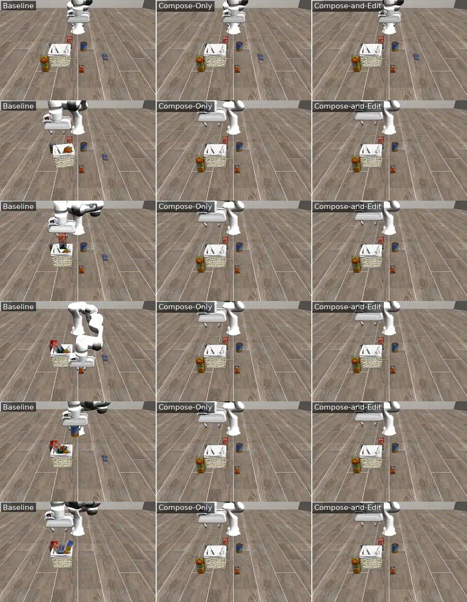
| Baseline4/10 · 247 s · 5.8/hr | Compose-Only9/10 · 46 s · 70.9/hr | Compose-and-Edit9/10 · 75 s · 43.0/hr |
“Pick the salad dressing and place it in the basket”
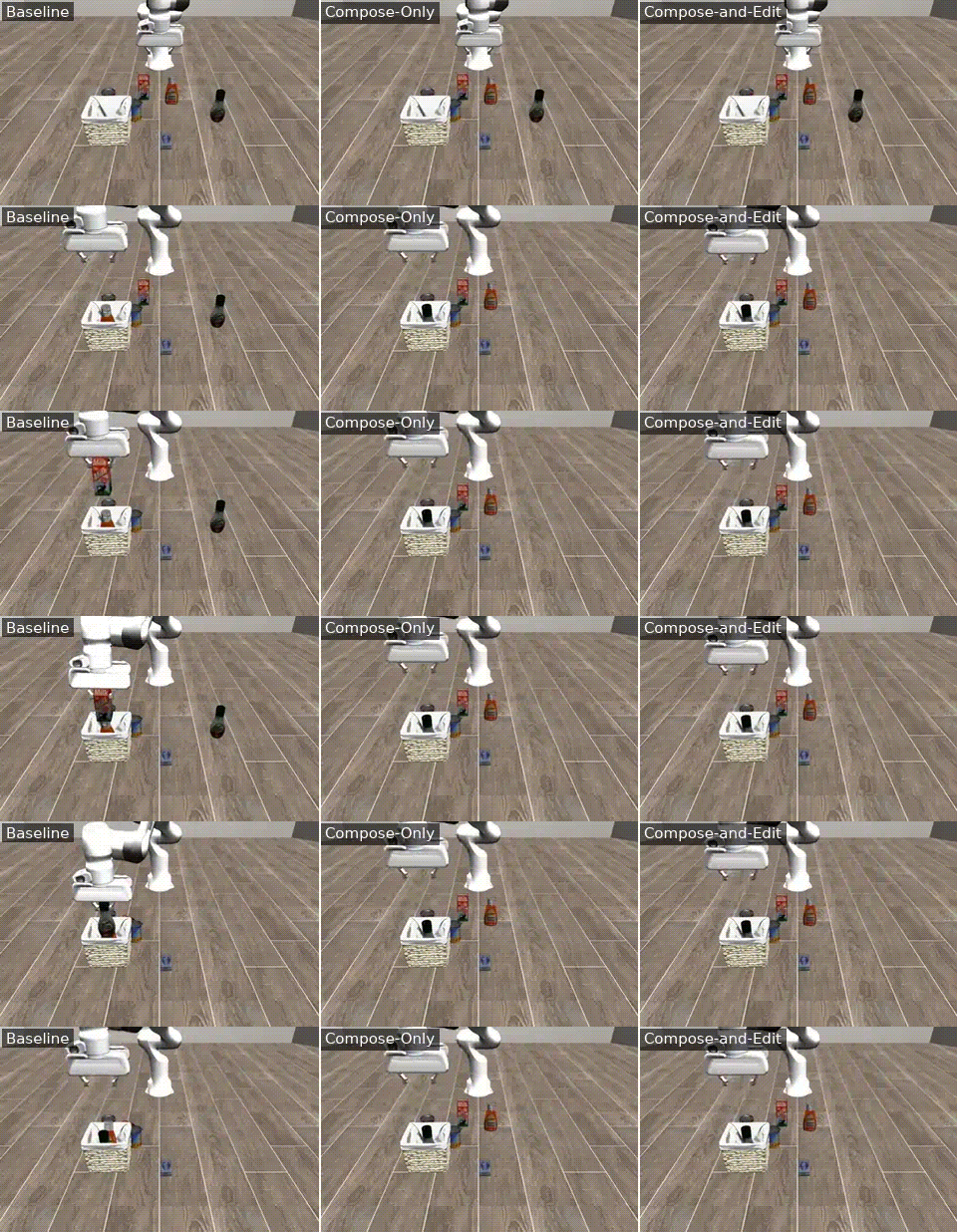
| Baseline3/10 · 163 s · 6.6/hr | Compose-Only10/10 · 34 s · 106.7/hr | Compose-and-Edit10/10 · 67 s · 53.5/hr |
“Pick the bbq sauce and place it in the basket”
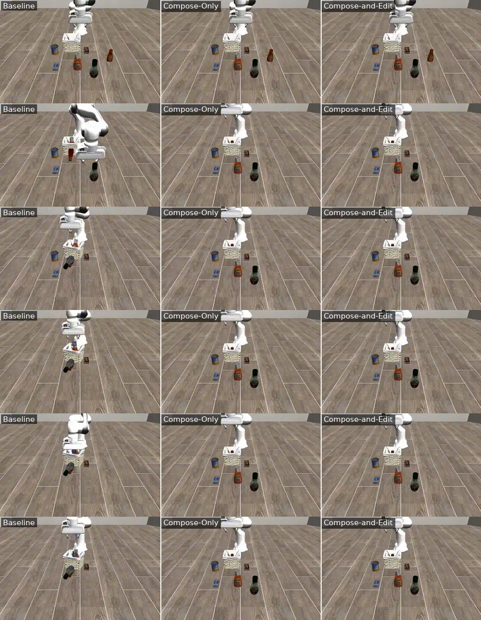
| Baseline8/10 · 95 s · 30.3/hr | Compose-Only9/10 · 33 s · 97.8/hr | Compose-and-Edit9/10 · 60 s · 54.0/hr |
“Pick the ketchup and place it in the basket”
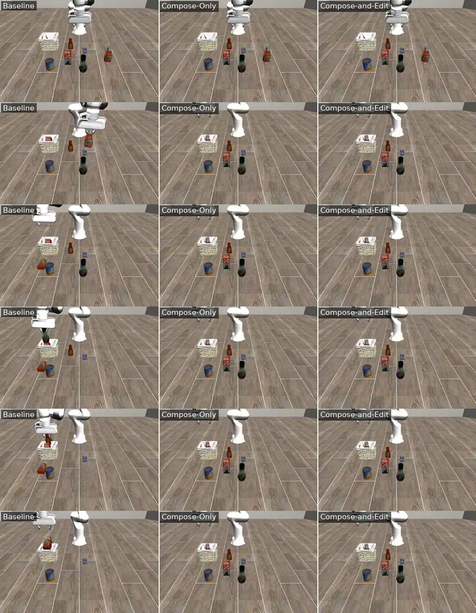
| Baseline8/10 · 117 s · 24.6/hr | Compose-Only10/10 · 35 s · 104.1/hr | Compose-and-Edit10/10 · 62 s · 57.9/hr |
“Pick the tomato sauce and place it in the basket”
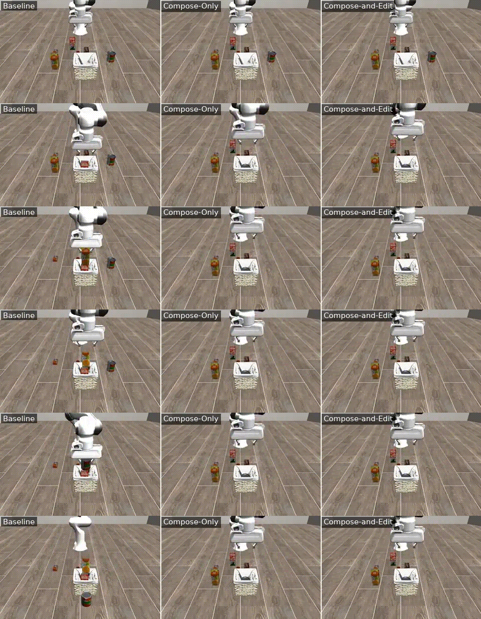
| Baseline8/10 · 133 s · 21.7/hr | Compose-Only10/10 · 35 s · 102.4/hr | Compose-and-Edit10/10 · 66 s · 54.5/hr |
“Pick the butter and place it in the basket”
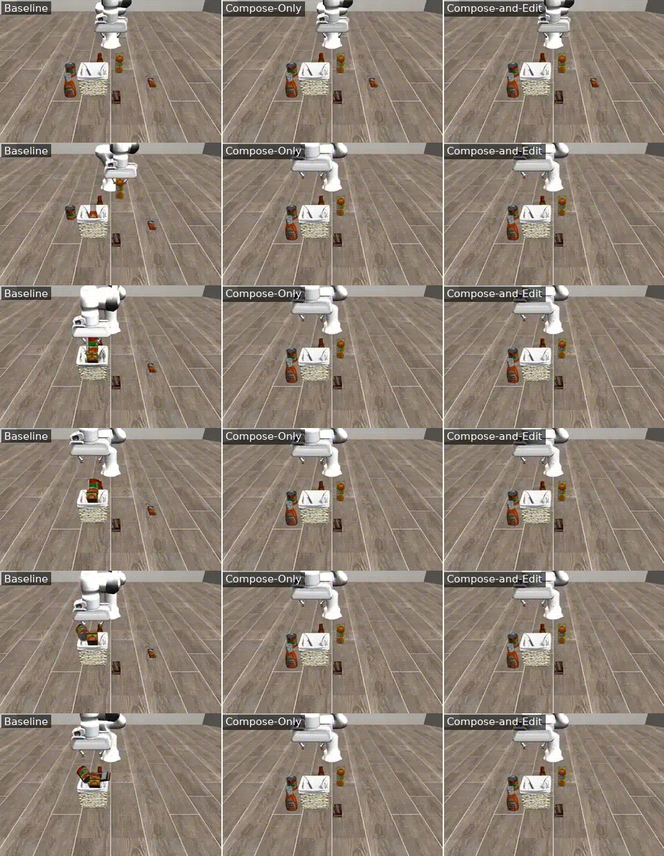
| Baseline5/10 · 220 s · 8.2/hr | Compose-Only9/10 · 55 s · 59.3/hr | Compose-and-Edit10/10 · 69 s · 52.3/hr |
“Pick the milk and place it in the basket”
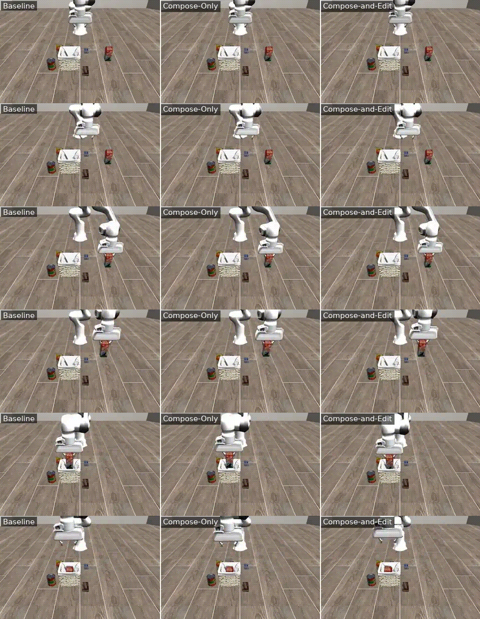
| Baseline10/10 · 52 s · 69.2/hr | Compose-Only10/10 · 36 s · 99.9/hr | Compose-and-Edit10/10 · 58 s · 62.1/hr |
“Pick the chocolate pudding and place it in the basket”
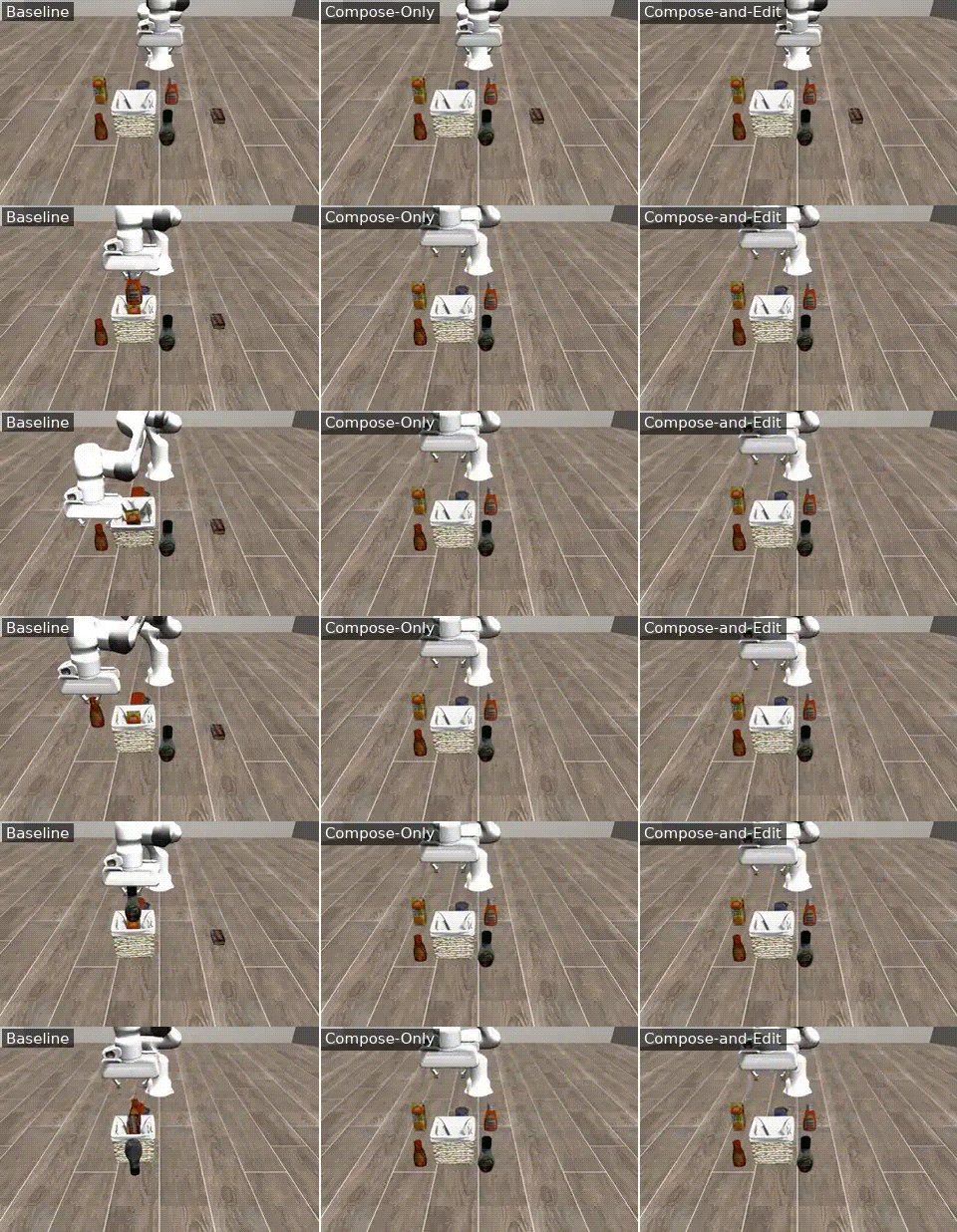
| Baseline5/10 · 216 s · 8.3/hr | Compose-Only10/10 · 45 s · 79.5/hr | Compose-and-Edit10/10 · 80 s · 45.1/hr |
“Pick the orange juice and place it in the basket”
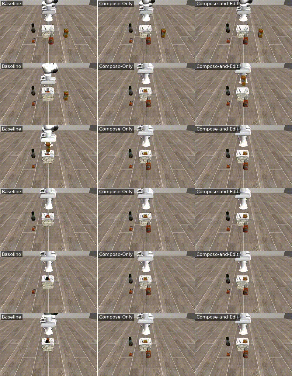
| Baseline6/10 · 88 s · 24.6/hr | Compose-Only10/10 · 32 s · 113.0/hr | Compose-and-Edit10/10 · 62 s · 57.7/hr |
“Pick all the objects and place them in the basket”
Ten scenes share this one instruction where each instance changes which objects are on the table. Scene 0 is shown; the figures below pool all ten. This is also the one row where Compose-Only runs longest, so the Baseline panel is the first to freeze. It still loses on throughput, if only barely 😎
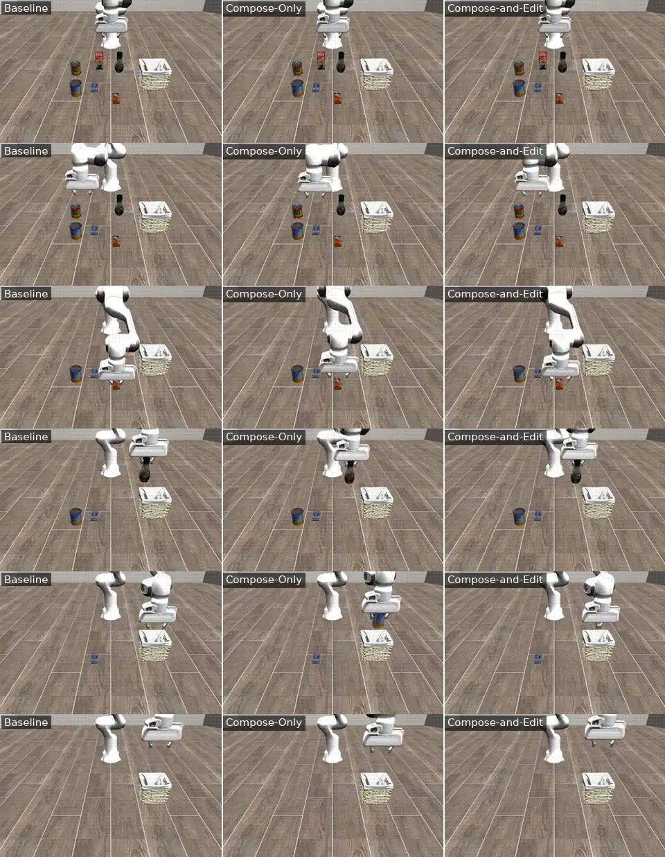
| Baseline100/100 · 180 s · 20.0/hr | Compose-Only100/100 · 166 s · 21.7/hr | Compose-and-Edit100/100 · 179 s · 20.1/hr |
On the pack-all task at the bottom, the baseline’s indiscriminate grabbing is exactly the right behaviour and costs it nothing — all three policies land within 8% of each other. So the gains come entirely from the single-item instructions.
Why it’s faster
I counted one loop iteration as one perceive_next.observe event in each trial’s own execution trace, across all 300 trials of the final measurement.
| Policy | Passes | Grasps | Checks | s / pass | s / trial |
|---|---|---|---|---|---|
| Baseline | 5.04 | 4.17 | none | 28.8 | 144.9 |
| Compose-and-Edit | 2.01 | 1.04 | none | 33.8 | 68.0 |
| Compose-Only | 1.04 | 1.04 | 0.98 | 37.9 | 39.4 |
Look at the fourth column. Per-iteration cost is worse for both searched policies: 28.8 seconds for the baseline against 33.8 and 37.9. They made the loop run fewer times, while spending slightly more inside each pass. Multiplying the two factors recovers the observed speedups:
Compose-Only     : 4.85x fewer iterations  x  0.76 per-iteration penalty  =  3.68x   (observed 3.68x)
Compose-and-Edit : 2.51x fewer iterations  x  0.85 per-iteration penalty  =  2.13x   (observed 2.13x)
The baseline’s pass count has a long right tail: a mean of 5.04, with trials running out to eighteen passes. Both searched policies are single spikes. Compose-Only ran exactly one perception pass in 98 of 100 trials, and Compose-and-Edit exactly two in 95 of 100.
The search agents wrote 126 lines in total. Two pieces matter.
Artifact one: disambiguation, worth roughly four grasps
The baseline asks for a generic grocery item, so it picks an arbitrary one. Compose-Only added a node that runs before perception and resolves the target out of the instruction:
# co/optimized/graphs/grocery_packing/scripts/task_context.py - 99 lines, new file
def run(ctx: NodeContext) -> Output:
    prompt = _normalise(os.environ.get("GAP_TASK_PROMPT", ""))
    item   = _requested_item(prompt)          # regex out of the sentence
    if not item:
        return {"object_name": _GENERIC_NAME,
                "object_description": _GENERIC_DESCRIPTION}
    description  = f"the requested packaged grocery item: {item}."
    description += " Never the wicker basket or storage container."
    return {"object_name": item, "object_description": description}
Its two outputs replace the two hardcoded strings in the perception node’s inputs. "grocery item" becomes "cream cheese", and the elimination game ends.
Compose-and-Edit reached the same capability without touching the graph. It edited the perception skill instead, adding a resolver inside the script and two parameters to switch it on:
# ce/optimized/skills/perceiving-objects/scripts/perceive_dino_vlm.py - edited in place
def _resolve_task_target(requested_name: str, enabled: bool) -> str:
    """Recover the named target from the task instruction."""
    prompt = os.environ.get("GAP_TASK_PROMPT", "").strip()
    ...

# called further down, gated by a new node parameter:
object_name = _resolve_task_target(object_name, resolve_task_target)
Neither search was told what was wrong.
Artifact two: the completion check, worth the gap between the two searched policies
Only Compose-Only found this one, and I think it accounts for most of the 1.71× between the two. Twenty-seven lines:
# co/optimized/graphs/grocery_packing/scripts/check_task_completion.py - 27 lines, new file
def run(ctx: NodeContext) -> Output:
    try:
        result    = ctx.tool("sim.check_success")
        completed = bool(result.get("task_completed"))
        return {"route": "complete" if completed else "continue",
                "task_completed": completed}
    except Exception as exc:
        # non-simulator connectors continue via perception
        return {"route": "continue", "task_completed": False}
The baseline and Compose-and-Edit have no equivalent at this point in the graph. Having placed the right item, they loop back and run a whole additional perception cycle (about 34 seconds) before their completion check can fire. Compose-Only asks, gets an answer, and exits.
The part that only works in simulation
The completion check calls sim.check_success, the simulator’s own goal predicate. The starting graph already polls it after every perception pass, so all three policies use it; Compose-Only just calls it earlier. A real robot has no such oracle. Without it, Compose-Only would take one extra perception pass per trial (about 38 seconds), which puts it at roughly ≈2.8× the baseline instead of 5.27×.
It would be interesting to adjust the graph to not rely on the simulator for termination, which would better reflect reality.
What I take from this
The main lesson for me is that it doesn’t much matter what form the robot policy takes, as long as it’s code. The same RHO loop has now worked on three pretty different kinds:
- Repositories on CaP-Bench: 64.33% on LIBERO-PRO, where π0.5 gets 13.20%, with no LLM calls at deployment.
- An LLM agent’s harness on RAI: held-out success from 23.5% to 44.3%.
- A Graph-as-Policy here: 5.27× the throughput.
RHO also transfers zero-shot to a real Franka and Kinova Gen3, with success rates up to 85% (17 of 20), even with objects it had never seen, placed somewhere new each time. The recipe is the same every time: hand a coding agent the policy’s source, score what it writes in simulation, and keep what works.
The two experiments here make the same point at a smaller scale. Whether the agent could only rewire the graph or could also rewrite skills, it found the same missing capability. Nobody pointed at the hardcoded string. The best part is that in all cases, we are using RHO to improve robotics policies without the need for human demonstration data 🤯
<pThese GaP results are simulation only, and part of the 5.27× throughput jump leans on a simulator-only completion check. As such, I'd like to point the search at the slowest parts of the graph. Per-iteration cost actually got worse for both searched policies, so I suspect there's a lot left on the table.

Leave a comment